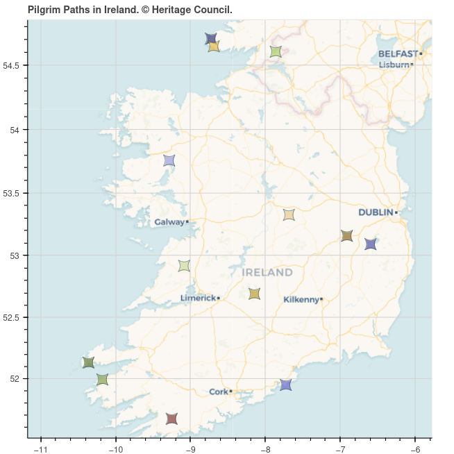
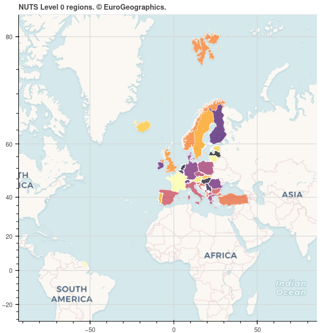
Bokeh is an open-source Python library for creating interactive visualisations that can be embedded into web pages. Here’s a Jupyter Notebook featuring an interactive map I made using Bokeh, showing pilgrim paths in Ireland, and here’s another one showing NUTS country-level boundaries. Hovering over each point on the map will show you the some metadata. On the right, there are controls to pan, zoom and reset the view, and also the option to save the current view as a PNG image.
Installing dependencies
The requirements are GeoPandas, JupyterLab, pooch, and Bokeh, as well as the jupyter_bokeh extension.
Make sure Python 3 is installed, then create a virtual environment using venv. Activate it and install all dependencies.
-
on Linux:
python -m venv env source env/bin/activate python -m pip install --upgrade pip setuptools wheel python -m pip install geopandas jupyterlab jupyter_bokeh pooch -
on Windows:
py -m venv env
.\env\Scripts\activate
py -m pip install --upgrade pip setuptools wheel
py -m pip install geopandas jupyterlab jupyter_bokeh pooch
Import libraries
In a Jupyter notebook, import the following libraries:
import os
from zipfile import ZipFile, BadZipFile

import geopandas as gpd
import pooch
import xyzservices.providers as xyz
from bokeh.io import output_notebook
from bokeh.models import CategoricalColorMapper, GeoJSONDataSource
from bokeh.palettes import Category20b, inferno
from bokeh.plotting import figure, show
Then, run the following to enable inline Bokeh plots:
output_notebook()
Plotting point data
Download the pilgrim paths dataset using Pooch:
FILE_NAME = "Pilgrim-Paths-Shapefiles.zip"
URL = f"https://www.heritagecouncil.ie/content/files/{FILE_NAME}"
KNOWN_HASH = None
SUB_DIR = os.path.join("data", "Pilgrim-Paths")
DATA_FILE = os.path.join(SUB_DIR, FILE_NAME)

# download data if necessary
if not os.path.isfile(os.path.join(SUB_DIR, FILE_NAME)):
    os.makedirs(SUB_DIR, exist_ok=True)
    pooch.retrieve(
        url=URL, known_hash=KNOWN_HASH, fname=FILE_NAME, path=SUB_DIR
    )
Read the pilgrim paths Shapefile data:
pilgrim_paths = gpd.read_file(
    f"zip://{DATA_FILE}!"
    + [x for x in ZipFile(DATA_FILE).namelist() if x.endswith(".shp")][0]
)
Since this dataset is in the Irish Transverse Mercator projection (EPSG:2157), while basemaps are in the Web Mercator projection (EPSG:3857), we need to reproject this dataset to EPSG:3857.
data = pilgrim_paths.to_crs(3857)
Note
The coordinates must be transformed into Web Mercator projection, as it is the projection used by map providers, such as OpenStreetMap and Google Maps, and if any of these providers are used as tiles for the plot without transforming the data, the mappings made by Bokeh will be inaccurate. See Wikipedia for more information about EPSG codes.
Bokeh requires the plot data to be in GeoJSON format, so convert it as follows:
geo_source = GeoJSONDataSource(geojson=data.to_json())
Generate unique colours for each point using a categorical colour palette:
const = list(set(data["Object_Typ"]))
palette = Category20b[len(const)]
color_map = CategoricalColorMapper(factors=const, palette=palette)
Define the plot title and tooltips:
TITLE = "Pilgrim Paths in Ireland. © Heritage Council."

TOOLTIPS = [
    ("Name", "@Object_Typ"),
    ("County", "@County"),
    ("Townland", "@Townland"),
    ("Start point", "@Start_Poin"),
    ("Length", "@Length_1"),
    ("Difficulty", "@Level_of_D"),
]
Configure the plot with map tools, tooltips, gridlines, and the title (the axes types are defined as mercator, so that the axes use latitudes and longitudes instead of Web Mercator coordinates):
p = figure(
    title=TITLE,
    tools="wheel_zoom, pan, reset, hover, save",
    tooltips=TOOLTIPS,
    x_axis_type="mercator",
    y_axis_type="mercator",
)

p.grid.grid_line_color = "lightgrey"

p.hover.point_policy = "follow_mouse"
Add the data points as a scatter plot:
p.scatter(
    "x",
    "y",
    source=geo_source,
    size=15,
    marker="square_pin",
    line_width=0.5,
    line_color="darkslategrey",
    fill_color={"field": "Object_Typ", "transform": color_map},
    fill_alpha=0.7,
)
Add a basemap:
p.add_tile(xyz.CartoDB.Voyager)
Finally, display the plot:
show(p)
See the interactive plot here!
Plotting polygon data
Download the NUTS dataset using Pooch:
FILE_NAME = "ref-nuts-2021-01m.shp.zip"
URL = (
    "https://gisco-services.ec.europa.eu/distribution/v2/nuts/download/"
    + FILE_NAME
)
SUB_DIR = os.path.join("data", "NUTS")
DATA_FILE = os.path.join(SUB_DIR, FILE_NAME)
os.makedirs(SUB_DIR, exist_ok=True)

# download data if necessary
if not os.path.isfile(os.path.join(SUB_DIR, FILE_NAME)):
    pooch.retrieve(
        url=URL, known_hash=KNOWN_HASH, fname=FILE_NAME, path=SUB_DIR
    )
Extract the archive:
try:
    z = ZipFile(DATA_FILE)
    z.extractall(SUB_DIR)
except BadZipFile:
    print("There were issues with the file", DATA_FILE)
Read the Level 0 data with Web Mercator projection:
DATA_FILE = os.path.join(SUB_DIR, "NUTS_RG_01M_2021_3857_LEVL_0.shp.zip")
nuts = gpd.read_file(f"zip://{DATA_FILE}!NUTS_RG_01M_2021_3857_LEVL_0.shp")
Convert the data to GeoJSON:
geo_source = GeoJSONDataSource(geojson=nuts.to_json())
Generate unique colours for each region using a continuous colour palette:
const = list(set(nuts["NUTS_ID"]))
palette = inferno(len(const))
color_map = CategoricalColorMapper(factors=const, palette=palette)
Define the plot title and tooltips:
TITLE = "NUTS Level 0 regions. © EuroGeographics."

TOOLTIPS = [
    ("Name", "@NAME_LATN"),
    ("NUTS Name", "@NUTS_NAME"),
    ("NUTS ID", "@NUTS_ID"),
    ("Country", "@CNTR_CODE"),
]
Configure the plot, add the data and a basemap, and display the plot:
p = figure(
    title=TITLE,
    tools="wheel_zoom, pan, reset, hover, save",
    tooltips=TOOLTIPS,
    x_axis_type="mercator",
    y_axis_type="mercator",
)

p.grid.grid_line_color = "lightgrey"

p.hover.point_policy = "follow_mouse"

# add data
p.patches(
    "xs",
    "ys",
    source=geo_source,
    line_width=0.5,
    line_color="white",
    fill_color={"field": "NUTS_ID", "transform": color_map},
    fill_alpha=0.7,
)

# add basemap
p.add_tile(xyz.CartoDB.Voyager)

show(p)
See the interactive map here!