https://www.met.ie/climate/available-data/mera
Summary
Issues with MÉRA GRIB 1 files when read using software packages such as the Xarray Python library:
- The data uses 0/360 longitude coordinates instead of -180/180
- data spans both negative and positive longitudes
- Projection information is present in the GRIB file but is not parsed when the data is read
- Lon/lat are multidimensional coordinates (y, x)
- data with two-dimensional coordinates cannot be spatially selected (e.g. extracting data for a certain point, or clipping with a geometry)
- x and y correspond to the index of the cells and are not coordinates in Lambert Conformal Conic projection
My solution:
- Use CDO to convert the GRIB 1 files to netCDF first
- projection info is parsed and can be read by Xarray
- one-dimensional coordinates in Lambert Conformal Conic projection
- data can now be indexed or selected both spatially and temporally using Xarray
- some metadata are lost (e.g. variable name and attributes) but these can be reassigned manually
- this method combines all three time steps in the example 3-h forecast data (data needs to be split prior to conversion to avoid this)
Relevant links:
- https://docs.xarray.dev/en/stable/examples/multidimensional-coords.html
- https://docs.xarray.dev/en/stable/examples/ERA5-GRIB-example.html
- https://cartopy.readthedocs.io/stable/reference/projections.html
- https://confluence.ecmwf.int/display/OIFS/How+to+convert+GRIB+to+netCDF
Requirements
Install the following in a Conda environment:
conda install --channel conda-forge python=3.10 cdo rioxarray cfgrib netcdf4 geopandas dask cartopy matplotlib nc-time-axis pooch
Procedure
Import libraries:
import os
from datetime import date, datetime, timezone
import cartopy.crs as ccrs
import geopandas as gpd
import matplotlib.dates as mdates
import matplotlib.pyplot as plt
import matplotlib.units as munits
import numpy as np
import pooch
import xarray as xr
Download sample data
Create a directory to store data:
DATA_DIR = os.path.join("data", "MERA", "sample")
os.makedirs(DATA_DIR, exist_ok=True)
Download sample GRIB data (2 m temperature; 3-h forecasts):
URL = "https://www.met.ie/downloads/MERA_PRODYEAR_2015_06_11_105_2_0_FC3hr.grb"
FILE_NAME = "MERA_PRODYEAR_2015_06_11_105_2_0_FC3hr"

if not os.path.isfile(os.path.join(DATA_DIR, FILE_NAME)):
    pooch.retrieve(
        url=URL,
        known_hash=None,
        fname=f"{FILE_NAME}.grb",
        path=DATA_DIR
    )

    with open(
        os.path.join(DATA_DIR, f"{FILE_NAME}.txt"), "w", encoding="utf-8"
    ) as outfile:
        outfile.write(
            f"Data downloaded on: {datetime.now(tz=timezone.utc)}\n"
            f"Download URL: {URL}"
        )
Path to the example data file:
BASE_FILE_NAME = os.path.join(DATA_DIR, FILE_NAME)
Read the original GRIB data
data = xr.open_dataset(
    f"{BASE_FILE_NAME}.grb",
    decode_coords="all", chunks="auto", engine="cfgrib"
)
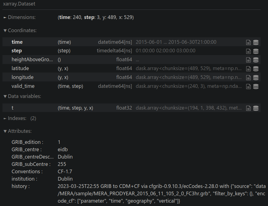
View the GRIB data:
data
Check if there’s any coordinate reference system (CRS) information in the data (there should be no output):
data.rio.crs
Save variable attributes for later:
t_attrs = data["t"].attrs
Convert longitude format
Convert 0/360 deg to -180/180 deg longitudes, and reassign attributes:
long_attrs = data.longitude.attrs
data = data.assign_coords(longitude=(((data.longitude + 180) % 360) - 180))
data.longitude.attrs = long_attrs
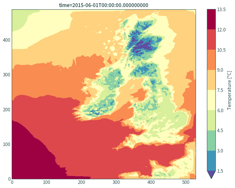
Visualise the data:
plt.figure(figsize=(9, 7))
(data.isel(time=0, step=2)["t"] - 273.15).plot.contourf(
robust=True, cmap="Spectral_r", levels=11,
cbar_kwargs={"label": "Temperature [°C]"}
)
plt.tight_layout()
plt.xlabel(None)
plt.ylabel(None)
plt.title(f"time={data.isel(time=0, step=2)['t']['time'].values}")
plt.show()
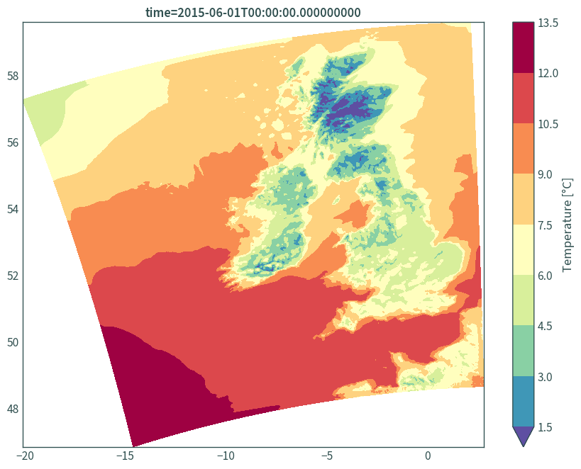
# use lon/lat
plt.figure(figsize=(9, 7))
(data.isel(time=0, step=2)["t"] - 273.15).plot.contourf(
robust=True, cmap="Spectral_r", x="longitude", y="latitude",
cbar_kwargs={"label": "Temperature [°C]"}, levels=11
)
plt.xlabel(None)
plt.ylabel(None)
plt.title(f"time={data.isel(time=0, step=2)['t']['time'].values}")
plt.tight_layout()
plt.show()
Convert GRIB to netCDF using CDO
Keeping only the third forecast step of the FC3hr data:
os.system(
    f"cdo -s -f nc4c -copy -seltimestep,3/{len(data['time']) * 3}/3 "
    f"{BASE_FILE_NAME}.grb {BASE_FILE_NAME}.nc"
)
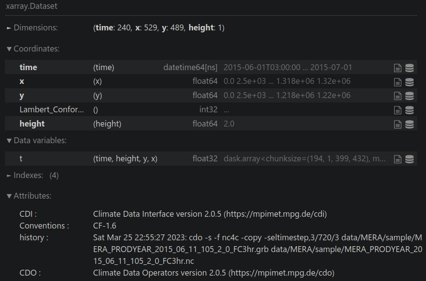
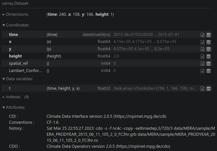
Read the netCDF file:
data = xr.open_dataset(
    f"{BASE_FILE_NAME}.nc", decode_coords="all", chunks="auto"
)
Reassign attributes and rename variables:
data["var11"].attrs = t_attrs
data = data.rename({"var11": "t"})
View the data:
data
View the CRS:
data.rio.crs
CRS.from_wkt('PROJCS["undefined",GEOGCS["undefined",DATUM["undefined",SPHEROID["undefined",6367470,0]],PRIMEM["Greenwich",0,AUTHORITY["EPSG","8901"]],UNIT["degree",0.0174532925199433]],PROJECTION["Lambert_Conformal_Conic_1SP"],PARAMETER["latitude_of_origin",53.5],PARAMETER["central_meridian",5],PARAMETER["scale_factor",1],PARAMETER["false_easting",1481641.67696368],PARAMETER["false_northing",537326.063885016],UNIT["metre",1,AUTHORITY["EPSG","9001"]],AXIS["Easting",EAST],AXIS["Northing",NORTH]]')
Plot using Lambert Conformal Conic projection
Define Lambert Conformal Conic projection for plots and transformations using metadata:
lambert_conformal = ccrs.LambertConformal(
    false_easting=data["Lambert_Conformal"].attrs["false_easting"],
    false_northing=data["Lambert_Conformal"].attrs["false_northing"],
    standard_parallels=[data["Lambert_Conformal"].attrs["standard_parallel"]],
    central_longitude=(
        data["Lambert_Conformal"].attrs["longitude_of_central_meridian"]
    ),
    central_latitude=(
        data["Lambert_Conformal"].attrs["latitude_of_projection_origin"]
    )
)
lambert_conformal
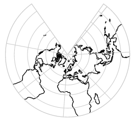
<cartopy.crs.LambertConformal object at 0x7fc44026b100>
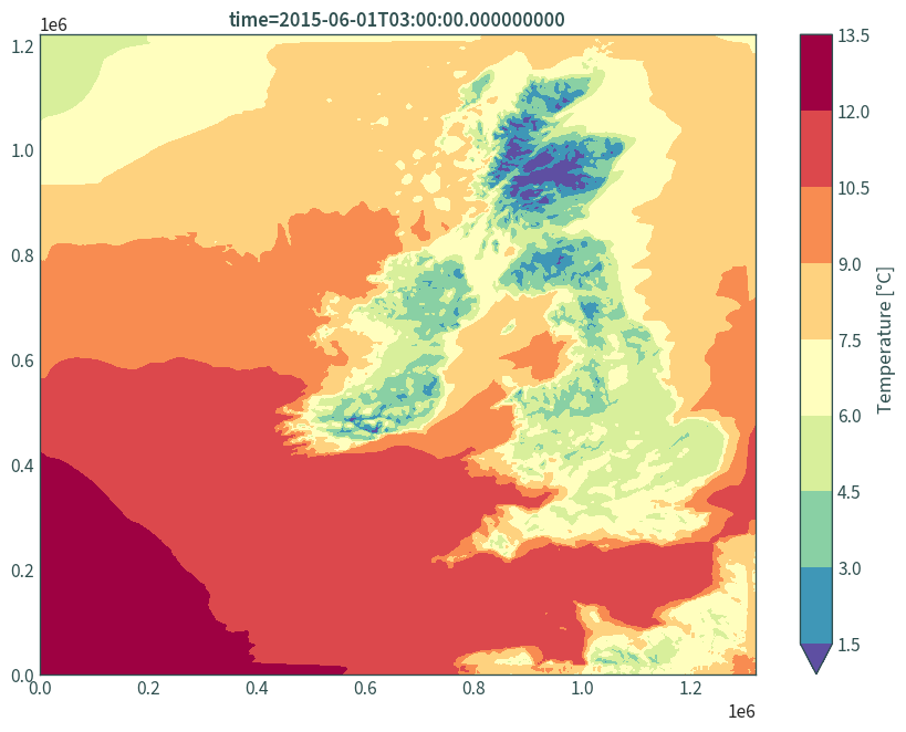
Plot data:
plt.figure(figsize=(9, 7))
(data.isel(time=0, height=0)["t"] - 273.15).plot.contourf(
robust=True, cmap="Spectral_r", levels=11,
cbar_kwargs={"label": "Temperature [°C]"}
)
plt.xlabel(None)
plt.ylabel(None)
plt.title(f"time={data.isel(time=0, height=0)['t']['time'].values}")
plt.tight_layout()
plt.show()
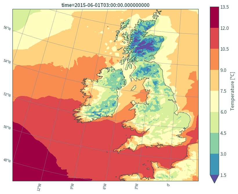
# in lon/lat
plt.figure(figsize=(9, 7))
ax = plt.axes(projection=lambert_conformal)
(data.isel(time=0, height=0)["t"] - 273.15).plot.contourf(
ax=ax, robust=True, cmap="Spectral_r", x="x", y="y", levels=11,
transform=lambert_conformal, cbar_kwargs={"label": "Temperature [°C]"}
)
ax.gridlines(
draw_labels={"bottom": "x", "left": "y"},
color="lightslategrey",
linewidth=.5,
x_inline=False,
y_inline=False
)
ax.coastlines(resolution="10m", color="darkslategrey", linewidth=.75)
plt.title(f"time={data.isel(time=0, height=0)['t']['time'].values}")
plt.tight_layout()
plt.show()
Clip to boundary of Ireland
Ireland boundary (derived from NUTS 2021):
ie = gpd.read_file(
  os.path.join("data", "boundary", "boundaries.gpkg"),
  layer="NUTS_RG_01M_2021_2157_IE"
)
Clip:
data_ie = data.rio.clip(
    ie.buffer(1).to_crs(lambert_conformal), all_touched=True
)
View data:
data_ie
Find number of grid cells with data:
len(
    data_ie.isel(time=0, height=0)["t"].values.flatten()[
        np.isfinite(data_ie.isel(time=0, height=0)["t"].values.flatten())
    ]
)
14490
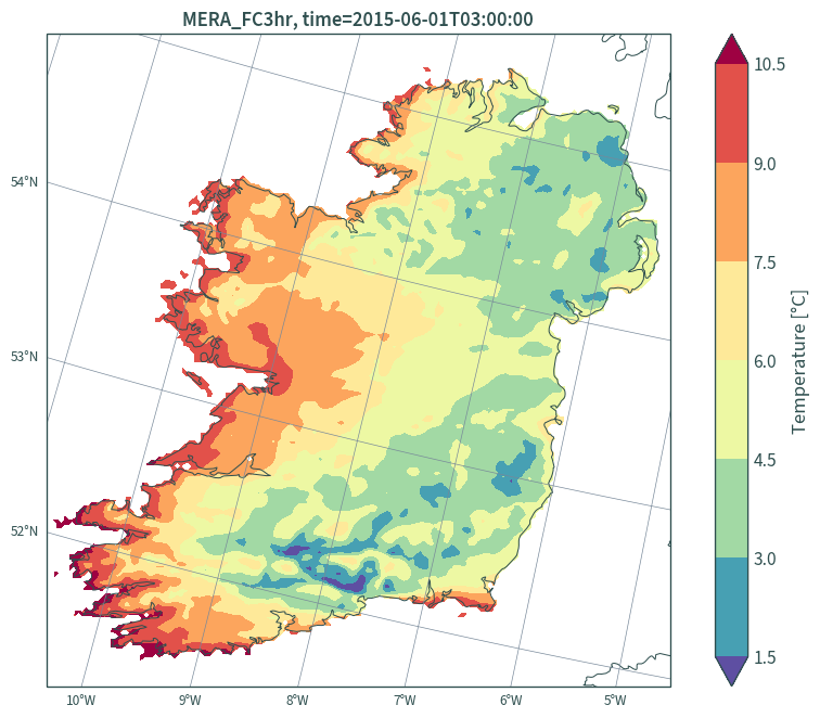
Plot:
plt.figure(figsize=(9, 7))
ax = plt.axes(projection=ccrs.EuroPP())
(data_ie.isel(time=0, height=0)["t"] - 273.15).plot.contourf(
    ax=ax, robust=True, cmap="Spectral_r", x="x", y="y", levels=8,
    transform=lambert_conformal, cbar_kwargs={"label": "Temperature [°C]"}
)
ax.gridlines(
    draw_labels={"bottom": "x", "left": "y"},
    color="lightslategrey",
    linewidth=.5,
    x_inline=False,
    y_inline=False
)
ax.coastlines(resolution="10m", color="darkslategrey", linewidth=.75)
plt.title(
    "MERA_FC3hr, " +
    f"time={str(data_ie.isel(time=0, height=0)['t']['time'].values)[:19]}"
)
plt.tight_layout()
plt.show()
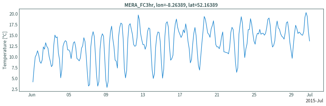
Extract time series for a grid point
Moorepark, Fermoy met station coordinates:
LON, LAT = -8.26389, 52.16389
Transform coordinates from lon/lat to Lambert Conformal Conic projection:
XLON, YLAT = lambert_conformal.transform_point(
    x=LON, y=LAT, src_crs=ccrs.PlateCarree()
)
XLON, YLAT
(579021.4574730808, 472854.55040691514)
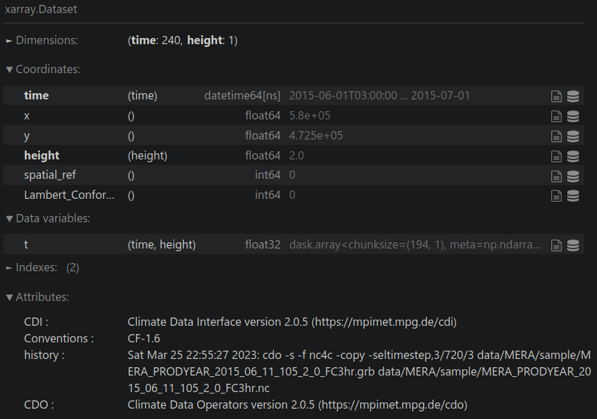
Extract data for the nearest grid cell to the point:
data_ts = data_ie.sel({"x": XLON, "y": YLAT}, method="nearest")
View data:
data_ts
Plot:
converter = mdates.ConciseDateConverter()
munits.registry[np.datetime64] = converter
munits.registry[date] = converter
munits.registry[datetime] = converter

plt.figure(figsize=(12, 4))
plt.plot(data_ts["time"], (data_ts["t"] - 273.15))
plt.ylabel("Temperature [°C]")
plt.title(f"MERA_FC3hr, lon={LON}, lat={LAT}")
plt.tight_layout()
plt.show()