Mapping pollen concentration across Great Britain using QGIS

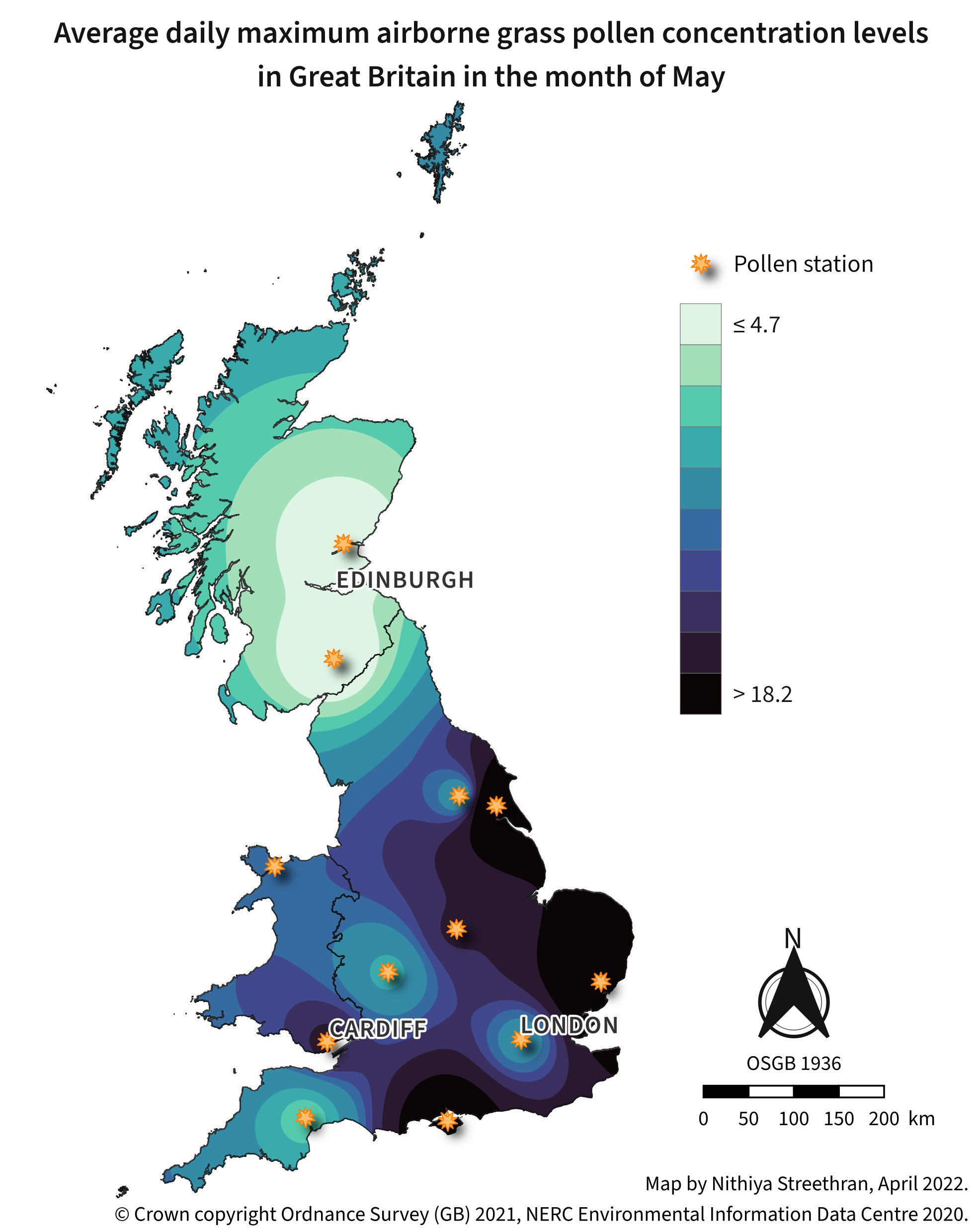
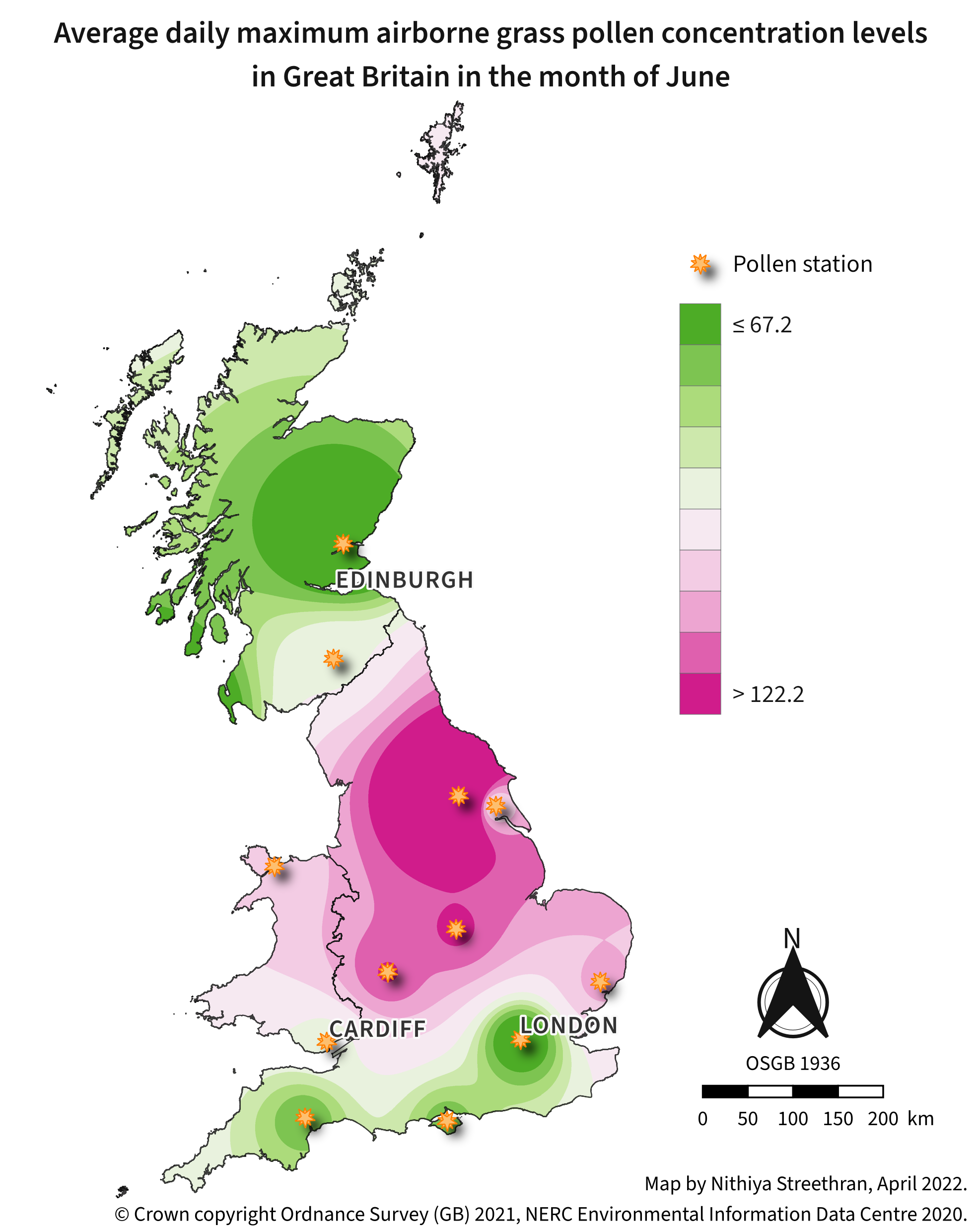
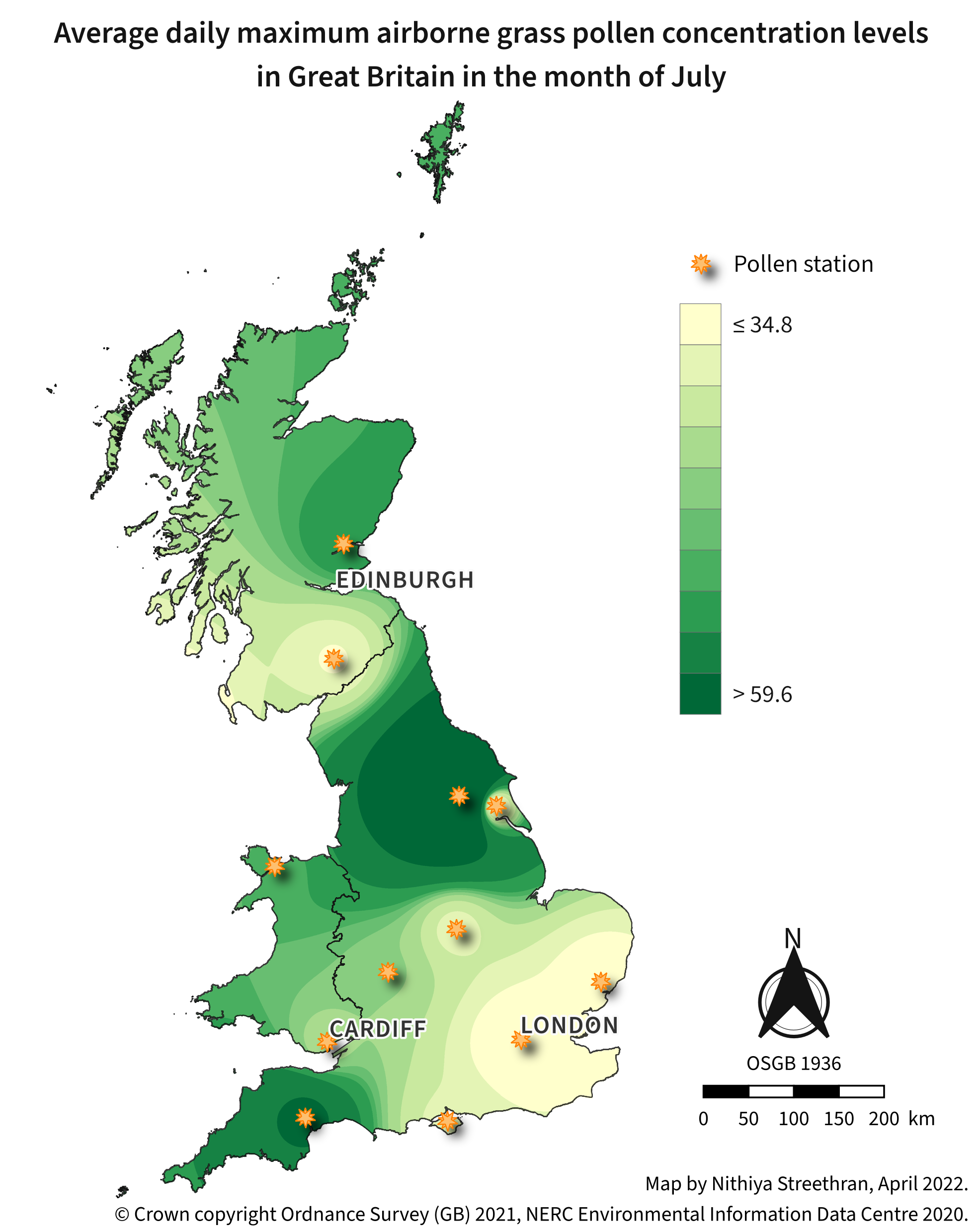
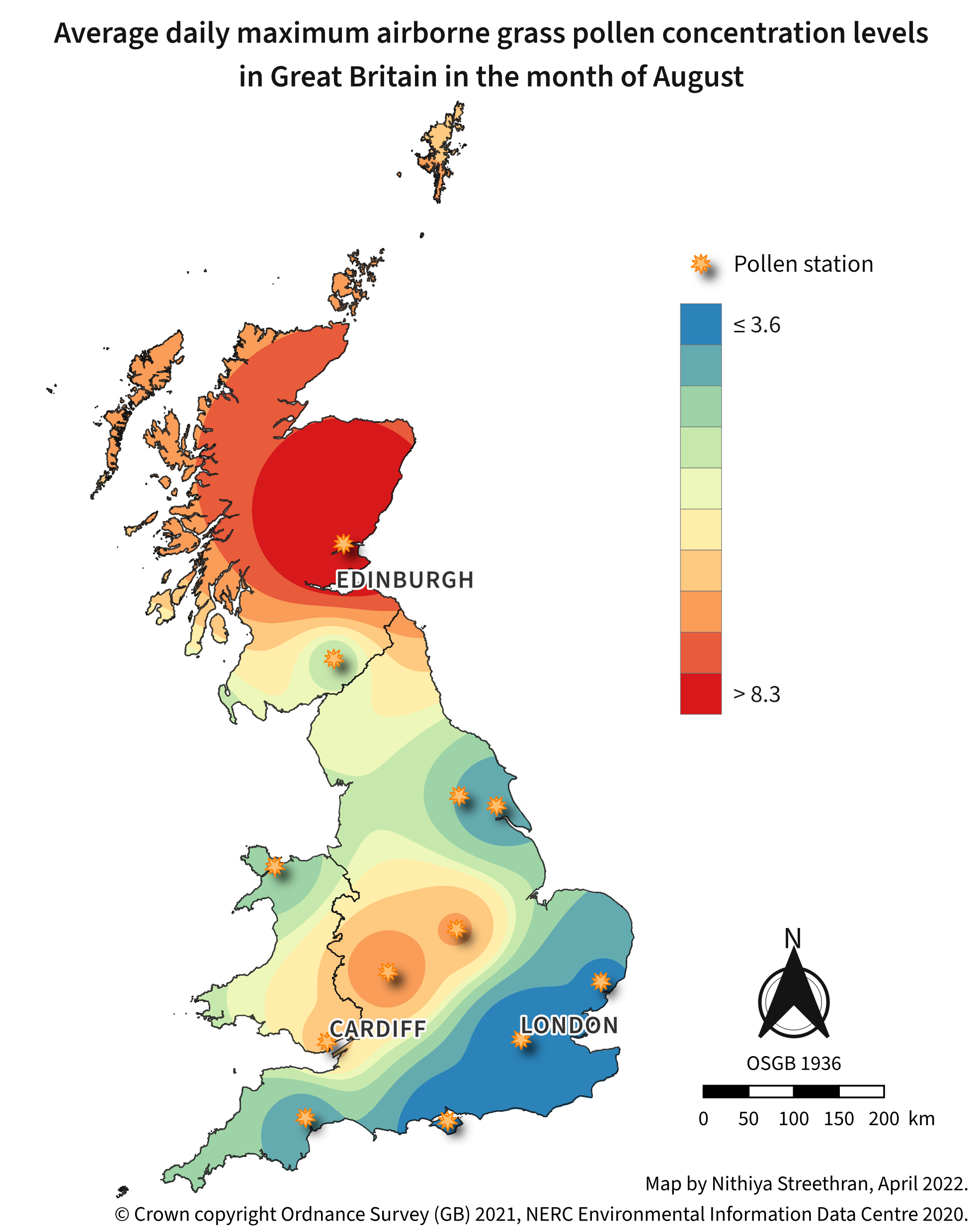
Airborne pollen concentration maps can be a useful indicator of areas to avoid during pollen season for people who suffer from hay fever¹.

Pollen concentration maps.

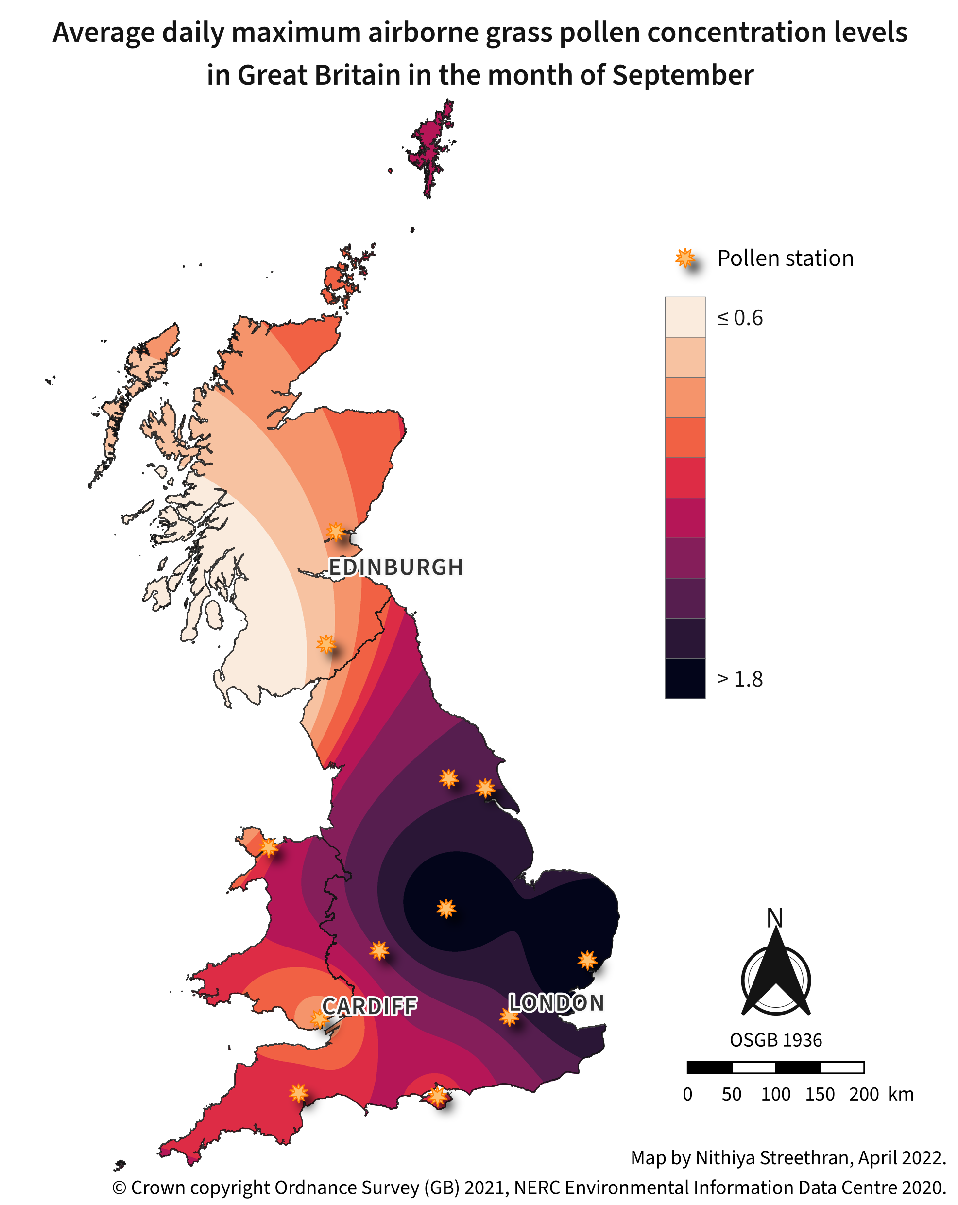
Tools used

Data (licenced under the Open Government Licence, version 3.0 (OGLv3.0)):

• Abundance of airborne pollen for nine grass species, measured by qPCR, UK, 2016-2017²
• OS Open Zoomstack, layer names³
• OS Boundary-Line™, layer country_region⁴

Software:

• QGIS
  • GDAL
• Python 3
  • Pandas
  • GeoPandas

Data processing

First, the pollen data must be restructured into a GeoPackage using the Python script shown in the section below.

The vector point data is interpolated using the Inverse Distance Weighted (IDW) algorithm in QGIS with the following Python snippet:

layerList = ["May", "Jun", "Jul", "Aug", "Sep"]
extent = (
    "5512.998000000,655989.000000000,5333.809600000,1220310.000000000" +
    " [EPSG:27700]"
)

for layer in layerList:
    interpolation_data = (
        "data/pollen-data.gpkg|layername=" + layer + "::~::0::~::16::~::0"
    )
    params = {
        "INTERPOLATION_DATA": interpolation_data,
        "EXTENT": extent,
        "PIXEL_SIZE": 100,
        "OUTPUT": "data/idw_" + layer + ".tif"
    }
    processing.run("qgis:idwinterpolation", params)

Each interpolated raster layer is then clipped to Great Britain’s boundary:

for layer in layerList:
    params = {
        "INPUT": "data/idw_" + layer + ".tif",
        "MASK": "data/bdline_gb.gpkg|layername=country_region",
        "SOURCE_CRS": QgsCoordinateReferenceSystem("EPSG:27700"),
        "TARGET_CRS": QgsCoordinateReferenceSystem("EPSG:27700"),
        "OUTPUT": "data/idw_" + layer + "_clipped.tif"
    }

    processing.run("gdal:cliprasterbymasklayer", params)

Mapping procedure

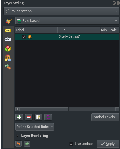
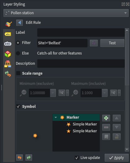
Pollen station point styling:

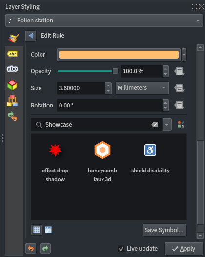
• Use a rule-based labelling to exclude Belfast using the filter Site!='Belfast'
• Use the ‘effect drop shadow’ symbol available in QGIS’ ‘Showcase’ point symbol list
• Change the fill colour to #fdbf6f and outline to #ff7f00

Point styling.

Basemap styling:

• Use OS stylesheets for the appropriate layers^{5 6}

• The stylesheets can be applied using the following process:

  # Open Zoomstack
  params = {
      "INPUT": "data/OS_Open_Zoomstack.gpkg|layername=names",
      "STYLE": "data/names.qml"
  }
  processing.run("native:setlayerstyle", params)
  
  # Boundary-Line
  params = {
      "INPUT": "data/bdline_gb.gpkg|layername=country_region",
      "STYLE": "data/country_region.qml"
  }
  processing.run("native:setlayerstyle", params)
  

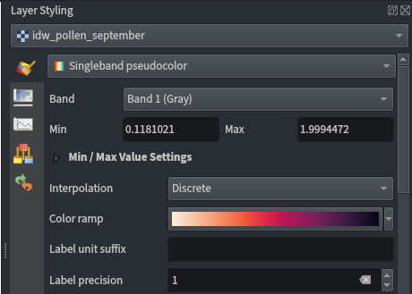
Raster layer styling:

• Singleband pseudocolour
• Discrete interpolation
• Label precision of 1
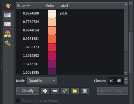
• Quantile classification mode
• 10 classes
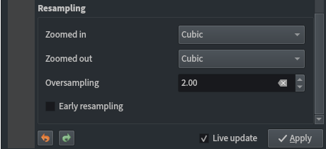
• Cubic resampling

Raster layer styling.

Raster colour ramps:

Raster colour ramps.

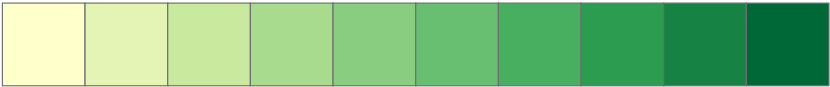
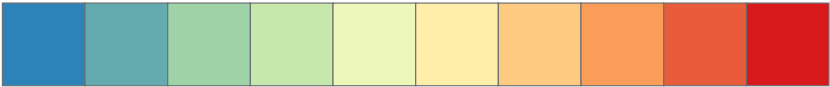
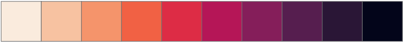
Mako and Rocket are Seaborn colour maps^{7 8}, while the rest are from ColorBrewer⁹.

Python script to restructure pollen data

# import libraries
import pandas as pd
import geopandas as gpd

# read data
pollen = pd.read_csv("data/qPCR_copy_number_abundance_data_aerial_DNA.csv")

# create well known text from coordinates
pollen["wkt"] = (
    "POINT (" + pollen["Long"].astype(str) + " " +
    pollen["Lat"].astype(str) + ")"
)

# drop cells with no value
pollen = pollen.dropna(subset=["Lat", "Long", "MaxPoaceaeConc", "year-month"])

# use full pollen monitoring site name
pollen = pollen.replace({
    "EXE": "Exeter", "EastR": "East Riding", "ESK": "Eskdalemuir",
    "LEIC": "Leicester", "CAR": "Cardiff", "IOW": "Isle of Wight",
    "IPS": "Ipswich", "BNG": "Bangor", "WOR": "Worcester",
    "KCL": "King's College London", "YORK": "York", "ING": "Invergowrie",
    "BEL": "Belfast"
})

# create a geo data frame
pollen = gpd.GeoDataFrame(
    pollen, geometry=gpd.GeoSeries.from_wkt(pollen["wkt"]), crs="EPSG:4326"
)

# drop unnecessary columns
pollen = pollen.drop(columns=["Lat", "Long", "wkt"])

# reproject to BNG
pollen = pollen.to_crs("epsg:27700")

# get list of months with available data
monthList = list(pollen["year-month"].str[0:3].unique())

# get list of pollen monitoring sites
pollen_sites = pollen[["Site", "geometry"]].drop_duplicates()

# aggregate monthly data for each site and save as GeoPackage layers
for m in monthList:
    pollen_month = pollen[pollen["year-month"].str.contains(m)]
    pollen_month = pollen_month.groupby(["Site"]).mean("MaxPoaceaeConc")
    pollen_month = pd.merge(pollen_month, pollen_sites, on="Site")
    pollen_month.to_file("data/pollen-data.gpkg", layer=m)

Footnotes

1. Met Office. 2022. Pollen Allergies. ↩

2. Brennan, G., S. Creer, and G. Griffith. 2020. Abundance of Airborne Pollen for Nine Grass Species, Measured by qPCR, UK, 2016-2017 [Dataset] [CSV]. NERC Environmental Information Data Centre. ↩

3. Ordnance Survey (GB). 2021. OS Open Zoomstack [Dataset] [GeoPackage] [v2021-12].. ↩

4. Ordnance Survey (GB). 2021. OS Boundary-Line™ [Dataset] [GeoPackage] [v2021-10]. ↩

5. Ordnance Survey (GB). 2021. OrdnanceSurvey/OS-Open-Zoomstack-Stylesheets/GeoPackage/QGIS Stylesheets (QML)/Outdoor style/names.qml.. GitHub. ↩

6. Ordnance Survey (GB). 2021. OrdnanceSurvey/Boundary-Line-stylesheets/Geopackage stylesheets/QGIS Stylesheets (QML)/country_region.qml. GitHub. ↩

7. Rudis, B., N. Ross, and S. Garnier. 2021. Introduction to the viridis color maps. ↩

8. Waskom, M. 2021. Choosing color palettes - seaborn 0.11.2 documentation. seaborn. ↩

9. Brewer, C. and M. Harrower. 2021. ColorBrewer: Color Advice for Maps. The Pennsylvania State University. ↩